1. 原子大模型排名
https://matbench-discovery.materialsproject.org/
2. 使用ASE结合mattersim进行结构优化、分子动力学
1. 使用ASE进行包括晶胞的结构优化
from mattersim.applications.moldyn import MolecularDynamics
from ase.io import read, write
from mattersim.forcefield import MatterSimCalculator
from mattersim.applications.relax import Relaxer
import numpy as np
from ase.optimize import LBFGS
from ase.filters import ExpCellFilter
from ase.io import Trajectory

# calc = MatterSimCalculator(device='cuda')
# calc = MatterSimCalculator(device='cuda:0')
calc = MatterSimCalculator(load_path="MatterSim-v1.0.0-5M.pth", device='cuda:0')

#relaxer = Relaxer(
#    optimizer="BFGS", # the optimization method FIRE, BFGS
#    filter=None, # filter to apply to the cell
#    constrain_symmetry=True, # whether to constrain the symmetry
#)

atoms = read("POSCAR",format='vasp')
atoms.calc = calc

ecf = ExpCellFilter(atoms)

traj = Trajectory('optimization.traj', 'w', atoms)
#converged, relaxed_structure = relaxer.relax_structures(atoms,optimizer="BFGS", # the optimization method FIRE, BFGS
#    filter=None,
#    constrain_symmetry=True, fmax=0.01 )
opt = LBFGS(ecf)
opt.attach(traj.write, interval=1)
opt.run(fmax=0.01)

write("POSCAR.vasp", atoms, format="vasp")
2. from wangq
from mattersim.applications.moldyn import MolecularDynamics
from ase.io import read, write
from mattersim.forcefield import MatterSimCalculator
from mattersim.applications.relax import Relaxer
import numpy as np

# calc = MatterSimCalculator(device='cuda')
calc = MatterSimCalculator(load_path="MatterSim-v1.0.0-5M.pth", device='cuda:2')
#默认是1M参数大模型,下面的是5M的

relaxer = Relaxer(
    optimizer="BFGS", # the optimization method FIRE, BFGS
    filter=None, # filter to apply to the cell
    constrain_symmetry=True, # whether to constrain the symmetry
)

atoms = read("SPOSCAR",format='vasp')
atoms.calc = calc

converged, relaxed_structure = relaxer.relax_structures(atoms,optimizer="FIRE", # the optimization method FIRE, BFGS
    filter=None,
    constrain_symmetry=True, fmax=0.1 )

# # 获取晶胞矩阵
# cell =   relaxed_structure.get_cell()

# # 尝试使用 Cholesky 分解将晶胞矩阵转换为上三角矩阵
# try:
#     # 确保晶胞矩阵是正定的
#     upper_triangular = np.linalg.cholesky(cell.dot(cell.T)).T
# except np.linalg.LinAlgError:
#     # 如果 Cholesky 分解失败,使用 QR 分解
#     _, upper_triangular = np.linalg.qr(cell)

# # 更新   relaxed_structure 对象的晶胞矩阵
# relaxed_structure.set_cell(upper_triangular, scale_atoms=True)

relaxed_structure.calc = calc

ensemble = "NVT_BERENDSEN"
temperature = 1000
timestep = 1.0
taut = 100
trajectory = "atoms.traj"
logfile = "atoms.log"
nvt_runner = MolecularDynamics(atoms=relaxed_structure, ensemble=ensemble, temperature=temperature, timestep=timestep, taut=taut, trajectory=trajectory, logfile = logfile)
nvt_runner.run(1000000)
3. 处理vaspkit 的MSD.dat得到电导率
import numpy as np
import matplotlib.pyplot as plt
from scipy.stats import linregress


def dealMSD(inputfile):
    data = np.loadtxt(inputfile,skiprows = 1 )
    data[:,0] = data[:,0] / 1000
    n = data.shape[0]
    start_idx = int(n*0.05)
    end_idx = int(n*0.95)
    time = data[start_idx:end_idx,0]
    MSD = data[start_idx:end_idx,4]
    slope, intercept, r_value, _, _ = linregress(time, MSD)
    MSD_fit = slope * time + intercept


    fig,ax1 = plt.subplots(figsize=(4,3),dpi = 600)
    ax1.plot(data[:, 0], data[:, 4],
            label='600 K',
            linewidth=2,          # 更粗的线条
            color='#2ecc71',      # 柔和的绿色
            alpha=0.8)
    ax1.plot(time, MSD_fit, label=f'Fit: y = {slope:.2f}x + {intercept:.2f}', color='red')
    ax1.set_xlabel('t (ps)')
    ax1.set_ylabel(r'MSD ($\AA^2$)')
    ax1.legend()
    ax1.grid(True)
    output_filename = inputfile.replace('/','-') + '.png'
    plt.savefig(output_filename, bbox_inches='tight')
    plt.close()
#    plt.show()
    return slope


diffD = []
temp = [600, 800,1000]
for i in temp:
    inputfile = f"{i}/msd/MSD.dat"
    try:
        slope = dealMSD(inputfile)
        diffuD = slope / 60000
        diffD.append(diffuD)
    except FileNotFoundError:
        print(f"文件 {inputfile} 不存在")
        diffD.append(0)
logdiffD = np.log10(diffD)
temp_inv = np.array([1000 / i for i in temp])


slope_D, intercept_D, _, _, _ = linregress(temp_inv, logdiffD)

temp_inv_fit = np.linspace(1, 3.3, 100)
logDfit = slope_D * temp_inv_fit + intercept_D
#logDfit = slope_D * temp_inv + intercept_D
fig,ax1 = plt.subplots(figsize=(4,3),dpi = 600)
ax1.plot(temp_inv_fit, logDfit, label=f'Fit: y = {slope_D:.2f}x + {intercept_D:.2f}', color='red')
ax1.scatter(temp_inv, logdiffD,color = 'blue',marker = 'o')
ax1.set_xlabel('1000/T (1/K)')
ax1.set_ylabel(r'log10(D) (Å$^2$/ps)')
ax1.set_xlim(0.9, 3.5)
ax1.set_ylim(slope_D * 3.5 + intercept_D, slope_D * 0.9 + intercept_D+ 0.3)

y_min = slope_D * 3.5 + intercept_D
y_max = slope_D * 0.9 + intercept_D + 0.3
y_ticks = np.arange(np.floor(y_min / 0.5) * 0.5, np.ceil(y_max / 0.5) * 0.5, 0.5)
ax1.set_yticks(y_ticks)

ax1.legend()
ax1.grid(True)
plt.savefig('arrnius.png',bbox_inches='tight')


from pymatgen.core import Structure
structure = Structure.from_file("POSCAR")
volume = structure.volume
atomsnumber = 30
Eanumber = 0.198691478
T = 300
logD300 = slope_D * (1000 / T) + intercept_D
D = 10 ** logD300

sigma300 = 1.858 * atomsnumber / volume / 300 * (10**12) * D
Ea = -Eanumber * slope_D

print(Ea, sigma300)
4. mattersim-MD直接输出MSD
from mattersim.applications.moldyn import MolecularDynamics
from ase.io import read, write
from mattersim.forcefield import MatterSimCalculator
from mattersim.applications.relax import Relaxer
import numpy as np
import os

# calc = MatterSimCalculator(device='cuda')
# calc = MatterSimCalculator(device='cuda:0')
calc = MatterSimCalculator(load_path="MatterSim-v1.0.0-1M.pth", device='cuda:0')

relaxer = Relaxer(
    optimizer="BFGS", # the optimization method FIRE, BFGS
    filter=None, # filter to apply to the cell
    constrain_symmetry=True, # whether to constrain the symmetry
)

atoms = read("POSCAR",format='vasp')
atoms.calc = calc

converged, relaxed_structure = relaxer.relax_structures(atoms,optimizer="BFGS", # the optimization method FIRE, BFGS
    filter=None,
    constrain_symmetry=True, fmax=0.01 )

# # 获取晶胞矩阵
# cell =   relaxed_structure.get_cell()

# # 尝试使用 Cholesky 分解将晶胞矩阵转换为上三角矩阵
# try:
#     # 确保晶胞矩阵是正定的
#     upper_triangular = np.linalg.cholesky(cell.dot(cell.T)).T
# except np.linalg.LinAlgError:
#     # 如果 Cholesky 分解失败,使用 QR 分解
#     _, upper_triangular = np.linalg.qr(cell)

# # 更新   relaxed_structure 对象的晶胞矩阵
# relaxed_structure.set_cell(upper_triangular, scale_atoms=True)


relaxed_structure.calc = calc
# import torch
# torch.cuda.empty_cache()

ensemble = "NVT_BERENDSEN"
temperature = 600
timestep = 2.0
taut = 100
trajectory = "atoms.traj"
logfile = "atoms.log"
nvt_runner = MolecularDynamics(atoms=relaxed_structure, ensemble=ensemble, temperature=temperature, timestep=timestep, taut=taut, trajectory=trajectory, loginterval=1,logfile = logfile)
nvt_runner.run(250000)


#将轨迹写入XDATCAR
atoms_xda = read('atoms.traj', index=':')
write('XDATCAR', atoms_xda)

os.remove('atoms.traj')


import numpy as np
import matplotlib
matplotlib.use("Agg")
import matplotlib.pyplot as plt

input_file = 'atoms.log'

data = np.loadtxt(input_file,skiprows=1)

fig,(ax1,ax2) = plt.subplots(1,2,figsize=(10,6),dpi=100)

ax1.plot(data[:, 0], data[:, 1],
         label='t-Energy',
         linewidth=2,          # 更粗的线条
         color='#2ecc71',      # 柔和的绿色
         alpha=0.8)            # 轻微的透明度
ax1.set_xlabel('t (ps)')
ax1.set_ylabel('Energy (eV)')
ax1.set_title('t-Energy')
ax1.legend()
ax1.grid(True)

ax2.plot(data[:, 0], data[:, 4],
         label='t-Temperature',
         linewidth=2,
         color='#e74c3c',      # 柔和的红色
         alpha=0.8)
ax2.set_xlabel('t (ps)')
ax2.set_ylabel('Temperature (K)')
ax2.set_title('t-Energy')
ax2.legend()
ax2.grid(True)


fig.tight_layout()

plot_file = 't-E-T.png'
fig.savefig(plot_file, dpi=300, bbox_inches='tight', facecolor='white')


#vaspkit处理
import subprocess

def run_vaspkit(task_id, selectype, element, skip_steps, frame_interval):
    # 构造VASPKIT命令
    command = f"(echo {task_id};echo {selectype};echo {element};echo {skip_steps};echo {frame_interval})| vaspkit"

    # 执行命令
    process = subprocess.Popen(command, shell=True, stdout=subprocess.PIPE, stderr=subprocess.PIPE)
    stdout, stderr = process.communicate()

    # 输出结果
    if process.returncode == 0:
        print("VASPKIT执行成功!")
        print(stdout.decode())
    else:
        print("VASPKIT执行失败!")
        print(stderr.decode())

# 示例调用
task_id = 722
selectype = 1
element = "Na"
skip_steps = 5000
frame_interval = 1

run_vaspkit(task_id, selectype, element, skip_steps, frame_interval)

if os.path.exists('MSD.dat'):
    os.remove('XDATCAR')
5. mattersim使用Nose-Hoover
from ase.io import read, write
from ase.optimize import BFGS
from ase.md.nose_hoover_chain import NoseHooverChainNVT
from ase import units
import numpy as np
import os
from ase.md.velocitydistribution import (
    MaxwellBoltzmannDistribution,
    Stationary,
)
from mattersim.forcefield import MatterSimCalculator

calc = MatterSimCalculator(load_path="MatterSim-v1.0.0-1M.pth", device='cuda:0')


atoms = read("POSCAR",format='vasp')
atoms.calc = calc

dyn = BFGS(atoms)
dyn.run(fmax=0.01)
write("optimized_structure.vasp", atoms)

temperature = 600
timestep = 2.0 * units.fs
tdamp = 100
trajectory = "atoms.traj"
logfile = "atoms.log"
loginterval = 1
append_trajectory = False


MaxwellBoltzmannDistribution(atoms,temperature_K=temperature,force_temp = True)

Stationary(atoms)

md1 = NoseHooverChainNVT(atoms=atoms,timestep=timestep,temperature_K = temperature,tdamp=tdamp,trajectory = None,logfile='equili.log',loginterval= loginterval,append_trajectory=append_trajectory)

md1.run(5000)

md2= NoseHooverChainNVT(atoms=atoms,timestep=timestep,temperature_K = temperature,tdamp=tdamp,trajectory = trajectory,logfile=logfile,loginterval= loginterval,append_trajectory=append_trajectory)

md2.run(5000)


#将轨迹写入XDATCAR
atoms_xda = read('atoms.traj', index=':')
write('XDATCAR', atoms_xda)

os.remove('atoms.traj')


import numpy as np
import matplotlib
matplotlib.use("Agg")
import matplotlib.pyplot as plt

input_file = 'atoms.log'

data = np.loadtxt(input_file,skiprows=1)

fig,(ax1,ax2) = plt.subplots(1,2,figsize=(10,6),dpi=100)

ax1.plot(data[:, 0], data[:, 1],
         label='t-Energy',
         linewidth=2,          # 更粗的线条
         color='#2ecc71',      # 柔和的绿色
         alpha=0.8)            # 轻微的透明度
ax1.set_xlabel('t (ps)')
ax1.set_ylabel('Energy (eV)')
ax1.set_title('t-Energy')
ax1.legend()
ax1.grid(True)

ax2.plot(data[:, 0], data[:, 4],
         label='t-Temperature',
         linewidth=2,
         color='#e74c3c',      # 柔和的红色
         alpha=0.8)
ax2.set_xlabel('t (ps)')
ax2.set_ylabel('Temperature (K)')
ax2.set_title('t-Energy')
ax2.legend()
ax2.grid(True)


fig.tight_layout()

plot_file = 't-E-T.png'
fig.savefig(plot_file, dpi=300, bbox_inches='tight', facecolor='white')


#vaspkit处理
import subprocess

def run_vaspkit(task_id, selectype, element, skip_steps, frame_interval):
    # 构造VASPKIT命令
    command = f"(echo {task_id};echo {selectype};echo {element};echo {skip_steps};echo {frame_interval})| vaspkit"

    # 执行命令
    process = subprocess.Popen(command, shell=True, stdout=subprocess.PIPE, stderr=subprocess.PIPE)
    stdout, stderr = process.communicate()

    # 输出结果
    if process.returncode == 0:
        print("VASPKIT执行成功!")
        print(stdout.decode())
    else:
        print("VASPKIT执行失败!")
        print(stderr.decode())

# 示例调用
task_id = 722
selectype = 1
element = "Na"
skip_steps = 5000
frame_interval = 1

run_vaspkit(task_id, selectype, element, skip_steps, frame_interval)

if os.path.exists('MSD.dat'):
    os.remove('XDATCAR')
6. 计算MSD 处理equili.log & atoms.log
import matplotlib.pyplot as plt
import matplotlib
import numpy as np
import os
from matplotlib import cm
from scipy.stats import linregress


matplotlib.use('Agg')


def ET(input_file, ax1,ax2):
    data = np.loadtxt(input_file,skiprows=1)
    ax1.plot(data[:, 0], data[:, 1],
            label='t-Energy',
            linewidth=2,          # 更粗的线条
            color='#2ecc71',      # 柔和的绿色
            alpha=0.8)            # 轻微的透明度
    ax1.set_xlabel('t (ps)')
    ax1.set_ylabel('Energy (eV)')
    ax1.set_title('t-Energy')
    ax1.legend()
    ax1.grid(True)

    ax2.plot(data[:, 0], data[:, 4],
            label='t-Temperature',
            linewidth=2,
            color='#e74c3c',      # 柔和的红色
            alpha=0.8)
    ax2.set_xlabel('t (ps)')
    ax2.set_ylabel('Temperature (K)')
    ax2.legend()
    ax2.grid(True)


def plottem(tem):
    data1 = np.loadtxt(os.path.join(base_folder, str(tem), 'MSD.dat'))
    data10 = data1[:, [0,4]]

    x = data10[:, 0] / 1000   # Convert time to ps and scale by 2 (example transformation)
    y_data = data10[:, 1]

    return x, y_data

def MSD_T(ax5):
    colors = cm.tab10
    # Plot data for each temperature
    for tem in tem_list:
        x, y_data = plottem(tem)

        n = x.shape[0]
        start_idx = int(n*0.05)
        end_idx = int(n*0.95)
        time = x[start_idx:end_idx]
        MSD = y_data[start_idx:end_idx]
        slope, intercept, r_value, _, _ = linregress(time, MSD)
        MSD_fit = slope * time + intercept

        color = colors.colors[int(tem /100)-4]
        ax5.plot(x, y_data,color=color, label=f'{tem} K',linewidth=2)
        ax5.plot(time, MSD_fit, color='red')
        ax5.set_xlabel('Time (ps)',fontsize=20, fontweight='bold')
        ax5.set_ylabel(r'MSD ($\mathrm{\AA}^2$)',fontsize=20,fontweight='bold')


        ax5.legend(prop={'weight':'bold','size':16})


def dealMSD(inputfile):
    data = np.loadtxt(inputfile,skiprows = 1 )
    data[:,0] = data[:,0] / 1000
    n = data.shape[0]
    start_idx = int(n*0.05)
    end_idx = int(n*0.95)
    time = data[start_idx:end_idx,0]
    MSD = data[start_idx:end_idx,4]
    slope, intercept, r_value, _, _ = linregress(time, MSD)
    MSD_fit = slope * time + intercept

    return slope


def arrniums(ax6):
    diffD = []

    for i in tem_list:
        inputfile = os.path.join(base_folder,str(i),'MSD.dat')
        try:
            slope = dealMSD(inputfile)
            diffuD = slope / 60000
            diffD.append(diffuD)
        except FileNotFoundError:
            print(f"文件 {inputfile} 不存在")
            diffD.append(0)
    logdiffD = np.log10(diffD)
    temp_inv = np.array([1000 / i for i in tem_list])


    slope_D, intercept_D, _, _, _ = linregress(temp_inv, logdiffD)

    temp_inv_fit = np.linspace(0.7, 3.3, 100)
    logDfit = slope_D * temp_inv_fit + intercept_D
    #logDfit = slope_D * temp_inv + intercept_D
    ax6.plot(temp_inv_fit, logDfit, label=f'Fit: y = {slope_D:.2f}x + {intercept_D:.2f}', color='red')
    ax6.scatter(temp_inv, logdiffD,color = 'blue',marker = 'o')
    ax6.set_xlabel('1000/T (1/K)')
    ax6.set_ylabel(r'log10(D) (Å$^2$/ps)')
    ax6.set_xlim(0.6, 3.5)
    ax6.set_ylim(slope_D * 3.5 + intercept_D, slope_D * 0.9 + intercept_D+ 0.3)

    y_min = slope_D * 3.5 + intercept_D
    y_max = slope_D * 0.7 + intercept_D + 0.3
    y_ticks = np.arange(np.floor(y_min / 0.5) * 0.5, np.ceil(y_max / 0.5) * 0.5, 0.5)
    ax6.set_yticks(y_ticks)

    ax6.legend()
    ax6.grid(True)
    # plt.savefig('arrnius.png',bbox_inches='tight')


    from pymatgen.core import Structure
    structure = Structure.from_file("POSCAR")
    num_atoms = structure.num_sites
    if num_atoms == 132:
        volume = structure.volume
        atomsnumber = 30
        Eanumber = 0.198691478
        T = 300
        logD300 = slope_D * (1000 / T) + intercept_D
        D = 10 ** logD300

        sigma300 = 1.858 * atomsnumber / volume / 300 * (10**12) * D
        Ea = -Eanumber * slope_D

        print(Ea, sigma300)


        text_str = f'Ea = {Ea:.2f}  eV\nSigma300K = {sigma300:.2f} mS/cm'
        ax6.text(0.95, 0.95, text_str, transform=ax6.transAxes,
                fontsize=10, verticalalignment='top', horizontalalignment='right',
                bbox=dict(facecolor='white', alpha=0.8, edgecolor='black'))

    else:
        print('not the 132 atoms cell')


def main():
    fig = plt.figure(figsize = (12,60), dpi = 300)
    gs = fig.add_gridspec(len(tem_list)* 2 + 1 ,2)
    ax1= fig.add_subplot(gs[0,0])
    ax2= fig.add_subplot(gs[0,1])
    MSD_T(ax1)
    arrniums(ax2)
    for idx, tem in enumerate(tem_list):
        row = idx*2 + 1
        equili_folder = os.path.join(base_folder,str(tem),'equili.log')
        atoms_folder = os.path.join(base_folder,str(tem),'atoms.log')
        ax_equili_T = fig.add_subplot(gs[row,0])
        ax_equili_E = fig.add_subplot(gs[row,1])
        ax_atoms_T = fig.add_subplot(gs[row+1,0])
        ax_atoms_E = fig.add_subplot(gs[row+1,1])
        ET(equili_folder,ax_equili_T,ax_equili_E)
        ET(atoms_folder,ax_atoms_T,ax_atoms_E)
        ax_equili_T.set_title(f'{tem} K')
    plt.tight_layout()
    plt.savefig('msd-TE.png')

base_folder = './'
tem_list = [600,800,1000,1200]

if __name__ == '__main__':
    main()
7. 处理不同次的MSD,得到所有MSD
# %%
import numpy as np
import os
import matplotlib.pyplot as plt
from matplotlib import cm
import matplotlib.font_manager as fm

base_folder = './'

def plottem(tem, msd_data_list):
    data1 = np.loadtxt(os.path.join(base_folder, str(tem), str(1), 'msd.dat'))
    data10 = data1[:, 0]
    msd_data_list.append(data10)
    for i in range(1, 4, 1):
        target_path = os.path.join(base_folder, str(tem), str(i), 'msd.dat')
        # print(target_path)
        data = np.loadtxt(target_path, skiprows=1)
        data_all = data[:, 4]
        data_all = data_all *132 / 30
        msd_data_list.append(data_all)

    # Padding to match the maximum length of data
    max_len = max(len(arr) for arr in msd_data_list)
    padded_data = np.array([np.pad(arr, (0, max_len - len(arr)), 'constant', constant_values=np.nan) for arr in msd_data_list])

    msd_data = padded_data.T
    x = msd_data[:, 0] / 1000 * 2  # Convert time to ps and scale by 2 (example transformation)
    y_data = msd_data[:, 1:]

    return x, y_data


plt.rcParams['font.family'] = 'Times New Roman'
plt.rcParams['font.size'] = 16
plt.rcParams['axes.linewidth'] = 2

plt.rcParams['axes.titlesize'] = 16
plt.rcParams['axes.labelsize'] = 20
plt.rcParams['axes.labelweight'] = 'bold'

plt.rcParams['xtick.labelsize'] = 16
plt.rcParams['ytick.labelsize'] = 16

plt.rcParams['legend.fontsize'] = 16


# Create the plot
plt.figure(figsize=(8, 6),dpi=300)
colors = cm.tab10
# Plot data for each temperature
for tem in [600, 700, 800, 900, 1000]:
    msd_data_list = []
    x, y_data = plottem(tem, msd_data_list)
    y_min = np.nanmin(y_data, axis=1)
    y_max = np.nanmax(y_data, axis=1)
    color = colors.colors[int(tem /100)-5]
    # Plot the curves for the current temperature
    for i in range(y_data.shape[1]):
        plt.plot(x, y_data[:, i],color=color, label=f'{tem} K' if i==0 else "")

    # Fill between the min and max values
    plt.fill_between(x, y_min, y_max, color=color, alpha=0.3)

# Final plot settings
plt.xlabel('Time (ps)')
plt.ylabel(r'MSD ($\mathrm{\AA}^2$)')


plt.xticks(fontweight = 'bold')
plt.yticks(fontweight = 'bold')
plt.legend(prop = {'weight' :'bold'})


plt.tight_layout()
# plt.show()
plt.savefig('888.png',dpi=600)
8.计算不同次分子动力学平均后的电导率
import numpy as np
import matplotlib.pyplot as plt
from scipy.stats import linregress


def dealMSD(inputfile):
    data = np.loadtxt(inputfile,skiprows = 1 )
    data[:,0] = data[:,0] / 1000 * 2
    n = data.shape[0]
    start_idx = int(n*0.05)
    end_idx = int(n*0.95)
    time = data[start_idx:end_idx,0]
    MSD = data[start_idx:end_idx,4]
    slope, intercept, r_value, _, _ = linregress(time, MSD)
    MSD_fit = slope * time + intercept


    fig,ax1 = plt.subplots(figsize=(4,3),dpi = 600)
    ax1.plot(data[:, 0], data[:, 4],
            label='600 K',
            linewidth=2,          # 更粗的线条
            color='#2ecc71',      # 柔和的绿色
            alpha=0.8)
    ax1.plot(time, MSD_fit, label=f'Fit: y = {slope:.2f}x + {intercept:.2f}', color='red')
    ax1.set_xlabel('t (ps)')
    ax1.set_ylabel(r'MSD ($\AA^2$)')
    ax1.legend()
    ax1.grid(True)
    output_filename = inputfile.replace('/','-') + '.png'
    plt.savefig(output_filename, bbox_inches='tight')
    plt.close()
#    plt.show()
    return slope


diffD = []
temp = [600, 700,800,900,1000]
for i in temp:
    diff_temp = []
    for j in [1,2,3]:
        inputfile = f"{i}/{j}/msd.dat"
        try:
            slope = dealMSD(inputfile)
            diffuD = slope / 60000
            diff_temp.append(diffuD)
            # diffD.append(diffuD)
        except FileNotFoundError:
            print(f"文件 {inputfile} 不存在")
            diff_temp.append(0)
    diff_temp = np.array(diff_temp)
    diff_temp_value = np.average(diff_temp)
    diffD.append(diff_temp_value)


logdiffD = np.log10(diffD)
temp_inv = np.array([1000 / i for i in temp])


slope_D, intercept_D, _, _, _ = linregress(temp_inv, logdiffD)

temp_inv_fit = np.linspace(1, 3.3, 100)
logDfit = slope_D * temp_inv_fit + intercept_D
#logDfit = slope_D * temp_inv + intercept_D
fig,ax1 = plt.subplots(figsize=(4,3),dpi = 600)
ax1.plot(temp_inv_fit, logDfit, label=f'Fit: y = {slope_D:.2f}x + {intercept_D:.2f}', color='red')
ax1.scatter(temp_inv, logdiffD,color = 'blue',marker = 'o')
ax1.set_xlabel('1000/T (1/K)')
ax1.set_ylabel(r'log10(D) (Å$^2$/ps)')
ax1.set_xlim(0.9, 3.5)
ax1.set_ylim(slope_D * 3.5 + intercept_D, slope_D * 0.9 + intercept_D+ 0.3)

y_min = slope_D * 3.5 + intercept_D
y_max = slope_D * 0.9 + intercept_D + 0.3
y_ticks = np.arange(np.floor(y_min / 0.5) * 0.5, np.ceil(y_max / 0.5) * 0.5, 0.5)
ax1.set_yticks(y_ticks)

ax1.legend()
ax1.grid(True)
plt.savefig('arrnius.png',bbox_inches='tight')


from pymatgen.core import Structure
structure = Structure.from_file("POSCAR")
volume = structure.volume
atomsnumber = 132
Eanumber = 0.198691478
T = 300
logD300 = slope_D * (1000 / T) + intercept_D
D = 10 ** logD300

sigma300 = 1.858 * atomsnumber / volume / 300 * (10**12) * D
Ea = -Eanumber * slope_D

print(Ea, sigma300)
3. 一些结果
大模型对NaInSiO的计算
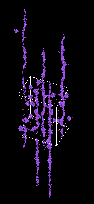
大模型能够比较好的模拟出Na的离子扩散行为
4. 一些脚本
1. 把ase轨迹转换为XDATCAR的脚本
使用ase自带的方法
ase convert --input-format traj --output-format vasp-xdatcar atoms.traj XDATCAR
python脚本
from ase.io import read, write

# 读取原始轨迹文件
atoms = read('atoms.traj', index=':')

# 将轨迹写入 XDATCAR 格式
write('XDATCAR', atoms)
2. 蒸馏大模型数据变成符合acnn标准的xsf文件的脚本
from mattersim.applications.moldyn import MolecularDynamics
from ase.io import read
from mattersim.forcefield import MatterSimCalculator
from mattersim.applications.relax import Relaxer
import numpy as np

# 使用 MatterSimCalculator 初始化计算器
calc = MatterSimCalculator(load_path="MatterSim-v1.0.0-5M.pth", device='cuda:0')

# 设置优化器
relaxer = Relaxer(
    optimizer="BFGS",  # 优化方法,使用 FIRE 或 BFGS
    filter=None,  # 是否应用过滤器
    constrain_symmetry=True,  # 是否约束对称性
)

# 读取 POSCAR 文件
atoms = read("POSCAR111.vasp", format='vasp')
atoms.calc = calc

# 进行结构弛豫
converged, relaxed_structure = relaxer.relax_structures(atoms, optimizer="FIRE", filter=None, constrain_symmetry=True, fmax=0.05)

# 设置计算器并准备进行分子动力学模拟
relaxed_structure.calc = calc

# 分子动力学参数
ensemble = "NVT_BERENDSEN"
temperature = 1000
timestep = 1.0
taut = 50
trajectory = "atoms.traj"
logfile = "atoms.log"
nvt_runner = MolecularDynamics(
    atoms=relaxed_structure,
    ensemble=ensemble,
    temperature=temperature,
    timestep=timestep,
    taut=taut,
    trajectory=trajectory,
    loginterval=1,
    logfile=logfile
)

# 保存每一帧为 .xsf 文件的函数
def write2my(file_path, ene_i, lat_i, ele_i, coo_i, foc_i):
    lat_i = lat_i.reshape(3, 3)
    coo_i = coo_i.reshape(-1, 3)
    foc_i = foc_i.reshape(-1, 3)
    with open(file_path, 'w') as file:
        file.write(f"# total energy = {ene_i} eV\n\n")
        file.write("CRYSTAL\n")
        file.write("PRIMVEC\n")

        for j in lat_i:
            for k in j:
                file.write(f'{k:20.8f}')
            file.write('\n')

        file.write("PRIMCOORD\n")
        file.write(f"{len(coo_i)} 1\n")

        for j in range(len(coo_i)):
            element_name = chemical_symbols[ele_i[j]]
            file.write(f'{element_name:2} ')
            # 写入坐标
            for k in coo_i[j]:
                file.write(f"{k:20.8f}")
            # 写入受力
            for k in foc_i[j]:
                file.write(f"{k:20.8f}")
            file.write("\n")

# 模拟运行并每50步保存一次 .xsf 文件
for step in range(1000000):  # 你可以根据需要设置步数
    nvt_runner.run(1)  # 运行一个步长
    atoms = nvt_runner.atoms  # 获取当前步长的原子对象

    # 每50步保存一次数据
    if step % 100 == 0:
        # 获取总能量
        energy = atoms.get_total_energy()

        # 获取晶胞矩阵
        cell = atoms.get_cell()

        # 获取原子元素类型
        atomic_numbers = atoms.get_atomic_numbers()

        # 获取原子坐标
        positions = atoms.get_positions()

        # 获取原子受力
        forces = atoms.get_forces()

        # 保存当前帧数据为 .xsf 文件
        frame_filename = f"frame_{step}.xsf"
        write2my(frame_filename, energy, cell, atomic_numbers, positions, forces)
3. 扩胞脚本
from pymatgen.io.vasp import Poscar

# 读取 POSCAR 文件
poscar = Poscar.from_file("POSCAR")

# 扩胞为 2x2x3
supercell = poscar.structure * [6, 6, 6]

# 将扩胞后的结构写入新的 POSCAR 文件
poscar = Poscar(supercell)
poscar.write_file("POSCAR666.vasp")
from ase.io import read,write
from ase.build import make_supercell
atoms = read("POSCAR")

P = [[3, 0, 0],
     [0, 3, 0],
     [0, 0, 3]]

supercell = make_supercell(atoms,P)
supercell.write("POSCAR333")
4. 计算体积脚本
from pymatgen.core import Structure

# 读取POSCAR文件
#structure = Structure.from_file("POSCAR.vasp")
structure = Structure.from_file("POSCAR.vasp")

# 计算体积
volume = structure.volume

# 输出体积
print(f"{volume} ų")
5. 元素替换脚本
import os
import shutil

# 创建文件夹
base_path = "./"  # 替换为你的根目录路径
element_symbols = ["La", "Ce","Pr","Nd","Pm","Eu","Sm","Gd","Tb","Dy","Ho","Er","Tm","Sc","Ti","V","Nb","Ta","Cr","Mo","Mn","Fe","Ru","Co","Rh","Ir","Ni","Pd","Cu","B","Al","Ga","In","N","P","Sb","Bi"]

for idx, element in enumerate(element_symbols, start=1):
    folder_name = f"{idx}-{element}"
    folder_path = os.path.join(base_path, folder_name)

    if not os.path.exists(folder_path):
        os.makedirs(folder_path)

# 读取原始 POSCAR 文件
input_file = "./POSCAR"  # 替换为你的 POSCAR 文件路径

with open(input_file, "r") as file:
    lines = file.readlines()

# 逐个元素进行替换并创建文件夹
for idx, element in enumerate(element_symbols, start=1):
    folder_name = f"{idx}-{element}"
    folder_path = os.path.join(base_path, folder_name)

    modified_lines = [line.replace("Y", element) for line in lines]

    # 写入修改后的内容到对应的文件夹
    output_file = os.path.join(folder_path, "POSCAR")
    with open(output_file, "w") as file:
        file.writelines(modified_lines)

    # 复制同名的 INCAR 文件到对应的文件夹
    incar_source = "./INCAR"  # 替换为你的 INCAR 文件路径
    incar_destination = os.path.join(folder_path, "INCAR")
    shutil.copy(incar_source, incar_destination)
    lsf_source = "./vasp.pbs"  # 替换为你的 INCAR 文件路径
    lsf_destination = os.path.join(folder_path, "opt.lsf")
    shutil.copy(lsf_source, lsf_destination)
print("Replacement and file writing complete.")
5. 使用m3gnet
# import warnings

# from m3gnet.models import Relaxer
# from pymatgen.core import Lattice, Structure
# from ase.io import read, write
# import tensorflow as tf
# from ase.optimize import BFGS

# for category in (UserWarning, DeprecationWarning):
#     warnings.filterwarnings("ignore", category=category, module="tensorflow")


# gpus = tf.config.list_physical_devices('GPU')
# if len(gpus) > 0:
#     tf.config.set_visible_devices(gpus[0], 'GPU')

# atoms = read("POSCAR222.vasp",format='vasp')

#  # 只使用第一块 GPU

# relaxer = Relaxer(optimizer = "BFGS")  # This loads the default pre-trained model

# relax_results = relaxer.relax(atoms,verbose=True)

# final_structure = relax_results['final_structure']
# final_energy_per_atom = float(relax_results['trajectory'].energies[-1] / len(atoms))

# print(f"Relaxed lattice parameter is {final_structure.lattice.abc[0]:.3f} Å")
# print(f"Final energy is {final_energy_per_atom:.3f} eV/atom")

from ase.optimize import BFGS
from m3gnet.models import Relaxer,M3GNetCalculator
from ase.io import read, write
import tensorflow as tf

gpus = tf.config.list_physical_devices('GPU')
if len(gpus) > 0:
    tf.config.set_visible_devices(gpus[0], 'GPU')

relaxer = Relaxer()
calculator = relaxer.calculator

atoms = read("POSCAR222.vasp",format='vasp')
# print(f"unrelaxed lattice parameter is {atoms.lattice.abc[0]:.3f} Å")
atoms.calc = calculator

optimizer = BFGS(atoms)

optimizer.run(fmax=0.01)

# print(f"Relaxed lattice parameter is {atoms.lattice.abc[0]:.3f} Å")
6. ASE结合phonopy 使用大模型作为计算器
1.关于声子谱
有限位移法(Finite Displacement Method)是一种用于计算晶体声子谱的数值方法,其基本原理是通过对晶体结构中的原子进行微小的位移,计算相应的力,从而构建力常数矩阵,进而求解声子频率和振动模式。

具体步骤如下:

结构优化:

首先,对晶体结构进行高精度的优化,以获得平衡的原子位置和晶格常数。
在优化过程中,需要设置适当的收敛标准,如能量收敛(EDIFF)和力收敛(EDIFFG)等,以确保结构的准确性。
构建超胞:

在优化后的结构基础上,使用Phonopy等工具构建超胞。
超胞的尺寸通常是原胞的整数倍,具体尺寸取决于所需的声子计算精度和计算资源。
原子位移:

对超胞中的每个原子进行微小的位移,通常在0.01到0.03埃之间。
这些位移可以是沿着晶体轴的正负方向,或者在不同方向上进行。
力计算:

在每个位移结构上,进行单点能量计算,获取每个原子所受的力。
这些力数据用于构建力常数矩阵。
构建力常数矩阵:

利用获得的力数据,构建力常数矩阵。
该矩阵描述了原子间的相互作用,是计算声子谱的基础。
声子谱计算:

通过对力常数矩阵进行对角化,得到声子的频率和振动模式。
进一步,可以绘制声子色散曲线,分析声子的行为。
注意事项:

有限位移法的计算精度高度依赖于力的计算精度,因此在结构优化和单点计算中需要设置严格的收敛标准。
位移幅度的选择需要平衡计算精度和计算量,过大的位移可能导致力常数矩阵的非线性,过小的位移可能导致数值误差。
计算过程中,可能需要考虑晶体的对称性,以减少计算量。
通过上述步骤,有限位移法能够有效地计算晶体的声子谱,为研究材料的热力学性质、动力学稳定性等提供重要信息。
2. 绘制投影声子态密度
import numpy as np
import matplotlib
matplotlib.use('Agg')
import matplotlib.pyplot as plt

# 读取文件
input_file1 = 'projected_dos.dat'  # 输入文件名
input_file2 = 'total_dos.dat'
output_file = 'tdosandpdos.dat'  # 输出文件名

# 读取数据
data = np.loadtxt(input_file1)
data2 = np.loadtxt(input_file2)

# 处理数据
# 第一列保持不变
col0 = data2[:,1]
col1 = data[:, 0]

# 第2-31列求和放到第二列
col2 = np.sum(data[:, 1:31], axis=1)

# 第32-37列求和放到第三列
col3 = np.sum(data[:, 31:37], axis=1)

# 第38-61列求和放到第四列
col4 = np.sum(data[:, 37:61], axis=1)

# 第62-133列求和放到第五列
col5 = np.sum(data[:, 61:133], axis=1)

# 将处理后的数据保存到新文件
processed_data = np.column_stack((col1, col2, col3, col4, col5,col0))
np.savetxt(output_file, processed_data, fmt='%.6f', delimiter='\t')


plt.figure(figsize=(10, 6), dpi=100)  # 增加 dpi 以提高分辨率

# 绘制图形,增强样式
plt.plot(processed_data[:, 0], processed_data[:, 1],
         label='PDOS_Na',
         linewidth=2,          # 更粗的线条
         color='#2ecc71',      # 柔和的绿色
         alpha=0.8)           # 轻微的透明度
plt.plot(processed_data[:, 0], processed_data[:, 2],
         label='PDOS_X',
         linewidth=2,
         color='#e74c3c',      # 柔和的红色
         alpha=0.8)
plt.plot(processed_data[:, 0], processed_data[:, 3],
         label='PDOS_Si',
         linewidth=2,
         color='#3498db',      # 柔和的蓝色
         alpha=0.8)
plt.plot(processed_data[:, 0], processed_data[:, 4],
         label='PDOS_O',
         linewidth=2,
         color='#9b59b6',      # 紫色
         alpha=0.8)
plt.plot(processed_data[:, 0], processed_data[:, 5],
         label='TDOS',
         linewidth=2.5,        # TDOS 线条稍粗
         color='#34495e',      # 深灰色
         alpha=0.9)

# 自定义坐标轴
plt.xlabel('ω (THz)', fontsize=12, labelpad=10)  # 使用希腊字母 ω 表示频率
plt.ylabel('Number', fontsize=12, labelpad=10)
plt.title('Partial and Total Density of States',
          fontsize=14,
          pad=15,
          fontweight='bold')

# 增强图例
plt.legend(
    fontsize=10,
    frameon=True,           # 添加边框
    framealpha=0.9,         # 轻微透明的边框
    edgecolor='gray',       # 边框颜色
    loc='best'              # 自动选择最佳位置
)

# 自定义网格(可选 - 浅色网格)
plt.grid(True, linestyle='--', alpha=0.3, color='gray')

# 调整边框(坐标轴边框)
ax = plt.gca()
ax.spines['top'].set_color('gray')
ax.spines['right'].set_color('gray')
ax.spines['left'].set_color('gray')
ax.spines['bottom'].set_color('gray')
ax.spines['top'].set_alpha(0.5)
ax.spines['right'].set_alpha(0.5)

# 添加次要刻度
plt.minorticks_on()

# 调整刻度参数
plt.tick_params(axis='both', which='major', labelsize=10)
plt.tick_params(axis='both', which='minor', length=2)

# 紧凑布局,防止标签被截断
plt.tight_layout()

# 保存高质量图像
plot_file = 'DOS.png'
plt.savefig(plot_file, dpi=300, bbox_inches='tight', facecolor='white')
7. ASE+grace
1. BFGS优化+NVTBerendsen分子动力学
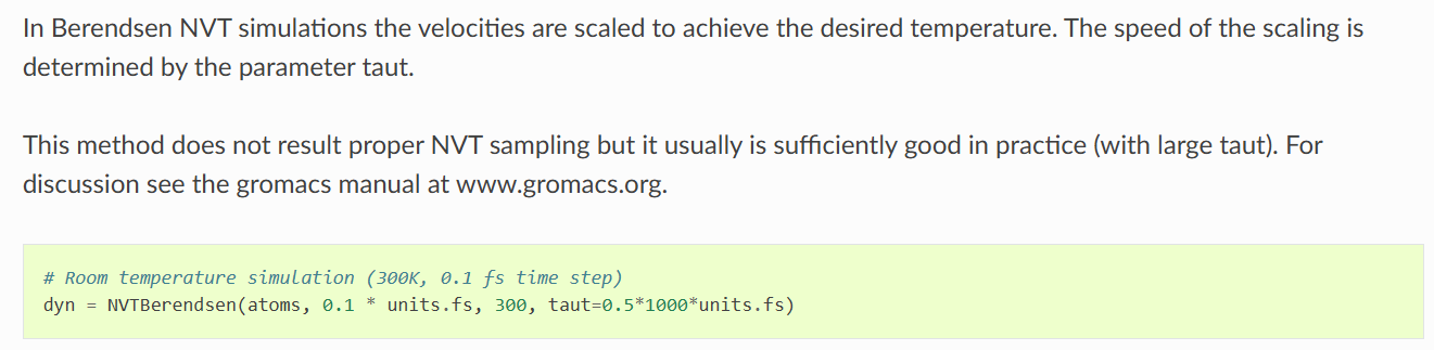
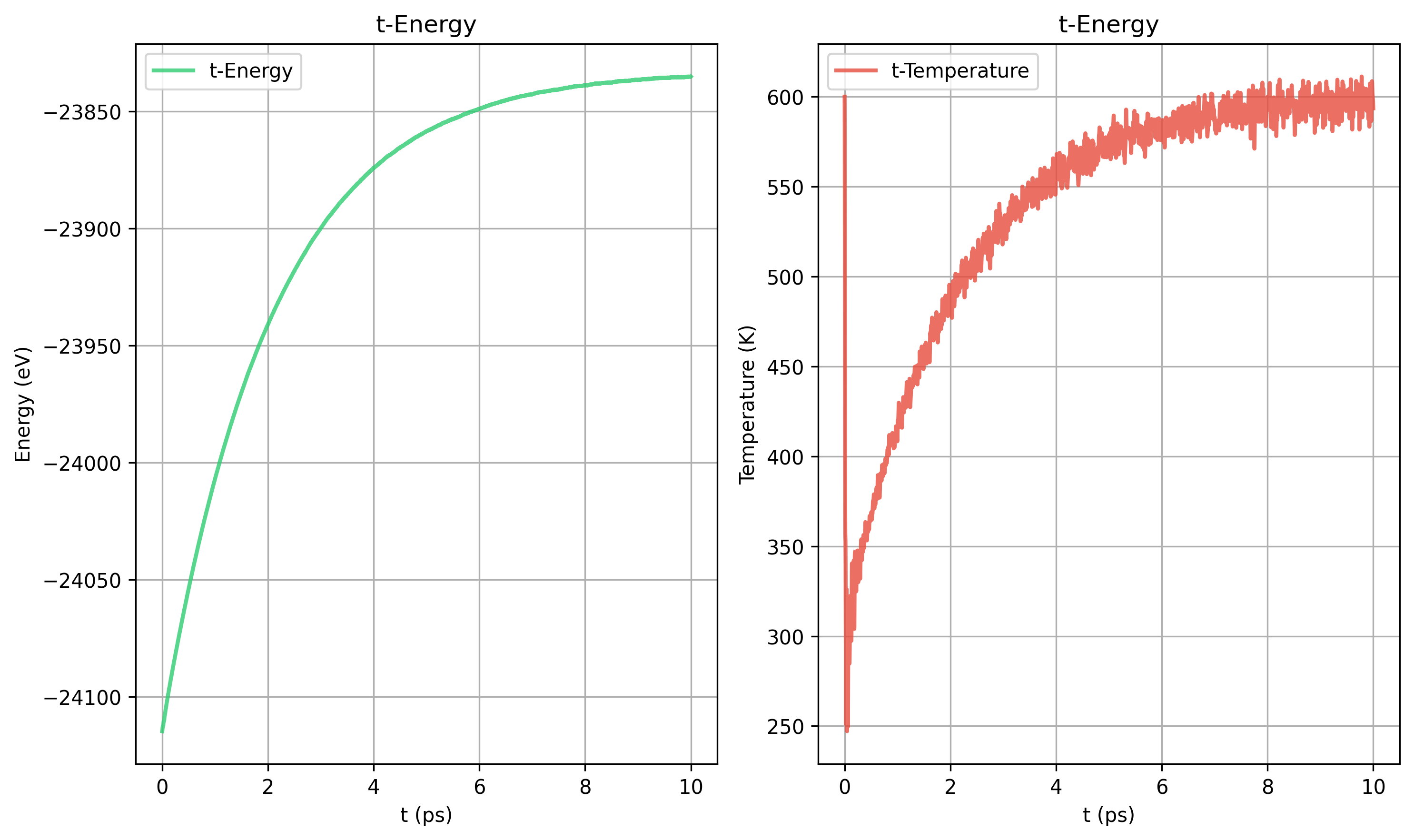
NVTBerendsen在taut比较小时可能得不到正确的动力学结果 ,因此模拟还是要用nose Hoover
from ase.io import read, write
from ase.optimize import BFGS
from ase.md.nvtberendsen import NVTBerendsen
from ase import units
from tensorpotential.calculator import grace_fm
import numpy as np
import os
from ase.md.velocitydistribution import (
    MaxwellBoltzmannDistribution,
    Stationary,
)

calc = grace_fm('GRACE-2L-OMAT')
atoms = read("POSCAR",format='vasp')
atoms.calc = calc

dyn = BFGS(atoms)
dyn.run(fmax=0.01)

temperature = 600
timestep = 2.0 * units.fs
taut = 100
trajectory = "atoms.traj"
logfile = "atoms.log"
loginterval = 1
append_trajectory = False


MaxwellBoltzmannDistribution(atoms,temperature_K=temperature,force_temp = True)

Stationary(atoms)

md = NVTBerendsen(atoms=atoms,timestep=timestep,temperature_K = temperature,taut=taut,trajectory = trajectory,logfile=logfile,loginterval= loginterval,append_trajectory=append_trajectory)

md.run(250000)


#后处理

#将轨迹写入XDATCAR
atoms_xda = read('atoms.traj', index=':')
write('XDATCAR', atoms_xda)

os.remove('atoms.traj')


import numpy as np
import matplotlib
matplotlib.use("Agg")
import matplotlib.pyplot as plt

input_file = 'atoms.log'

data = np.loadtxt(input_file,skiprows=1)

fig,(ax1,ax2) = plt.subplots(1,2,figsize=(10,6),dpi=100)

ax1.plot(data[:, 0], data[:, 1],
         label='t-Energy',
         linewidth=2,          # 更粗的线条
         color='#2ecc71',      # 柔和的绿色
         alpha=0.8)            # 轻微的透明度
ax1.set_xlabel('t (ps)')
ax1.set_ylabel('Energy (eV)')
ax1.set_title('t-Energy')
ax1.legend()
ax1.grid(True)

ax2.plot(data[:, 0], data[:, 4],
         label='t-Temperature',
         linewidth=2,
         color='#e74c3c',      # 柔和的红色
         alpha=0.8)
ax2.set_xlabel('t (ps)')
ax2.set_ylabel('Temperature (K)')
ax2.set_title('t-Energy')
ax2.legend()
ax2.grid(True)


fig.tight_layout()

plot_file = 't-E-T.png'
fig.savefig(plot_file, dpi=300, bbox_inches='tight', facecolor='white')


#vaspkit处理
import subprocess

def run_vaspkit(task_id, selectype, element, skip_steps, frame_interval):
    # 构造VASPKIT命令
    command = f"(echo {task_id};echo {selectype};echo {element};echo {skip_steps};echo {frame_interval})| vaspkit"

    # 执行命令
    process = subprocess.Popen(command, shell=True, stdout=subprocess.PIPE, stderr=subprocess.PIPE)
    stdout, stderr = process.communicate()

    # 输出结果
    if process.returncode == 0:
        print("VASPKIT执行成功!")
        print(stdout.decode())
    else:
        print("VASPKIT执行失败!")
        print(stderr.decode())

# 示例调用
task_id = 722
selectype = 1
element = "Na"
skip_steps = 5000
frame_interval = 1

run_vaspkit(task_id, selectype, element, skip_steps, frame_interval)

if os.path.exists('MSD.dat'):
    os.remove('XDATCAR')
2. 使用ASE中的Nose-Hoover NVT
from ase.io import read, write
from ase.optimize import BFGS
from ase.md.nose_hoover_chain import NoseHooverChainNVT
from ase import units
from tensorpotential.calculator import grace_fm
import numpy as np
import os
from ase.md.velocitydistribution import (
    MaxwellBoltzmannDistribution,
    Stationary,
)

calc = grace_fm('GRACE-2L-OMAT')
atoms = read("POSCAR",format='vasp')
atoms.calc = calc

dyn = BFGS(atoms)
dyn.run(fmax=0.01)
write("optimized_structure.vasp", atoms)

temperature = 600
timestep = 2.0 * units.fs
tdamp = 100
trajectory = "atoms.traj"
logfile = "atoms.log"
loginterval = 1
append_trajectory = False


MaxwellBoltzmannDistribution(atoms,temperature_K=temperature,force_temp = True)

Stationary(atoms)

md1 = NoseHooverChainNVT(atoms=atoms,timestep=timestep,temperature_K = temperature,tdamp=tdamp,trajectory = None,logfile='equili.log',loginterval= loginterval,append_trajectory=append_trajectory)

md1.run(10000)

md2= NoseHooverChainNVT(atoms=atoms,timestep=timestep,temperature_K = temperature,tdamp=tdamp,trajectory = trajectory,logfile=logfile,loginterval= loginterval,append_trajectory=append_trajectory)

md2.run(250000)
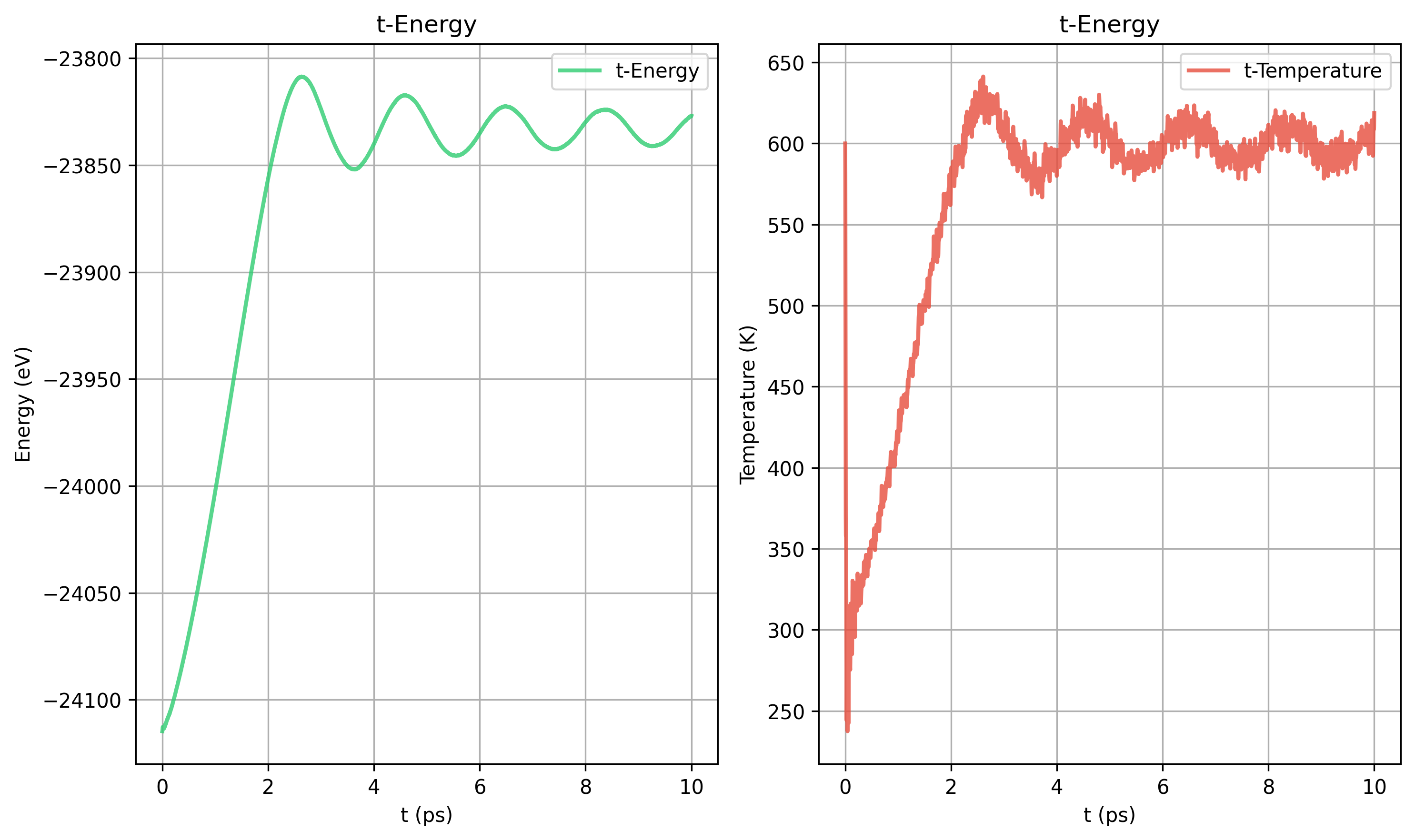
8. Nose-Hoover和Berendsen的对比
更大的晶胞也需要更长的弛豫时间
Nose-Hoover tdamp= 200 vs Berendsen taut=100
Nose-Hoover和Berendsen的动力学过程不同
Nose-Hoover

Berendsen
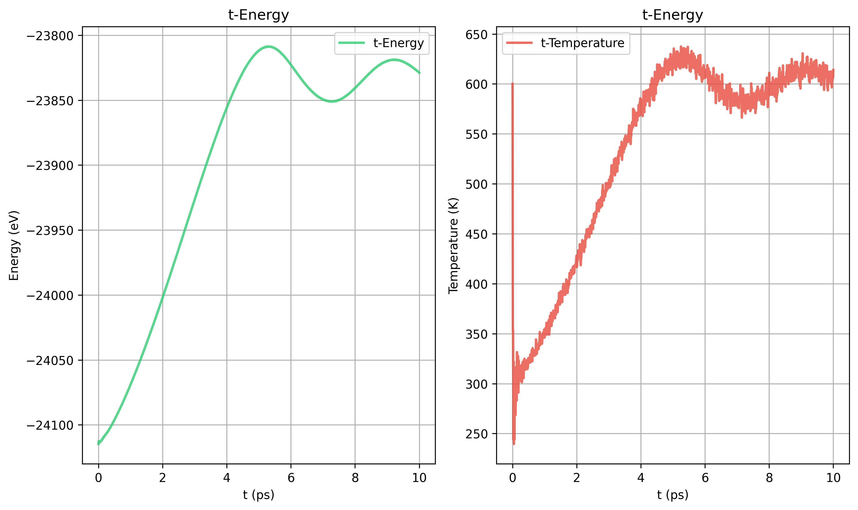
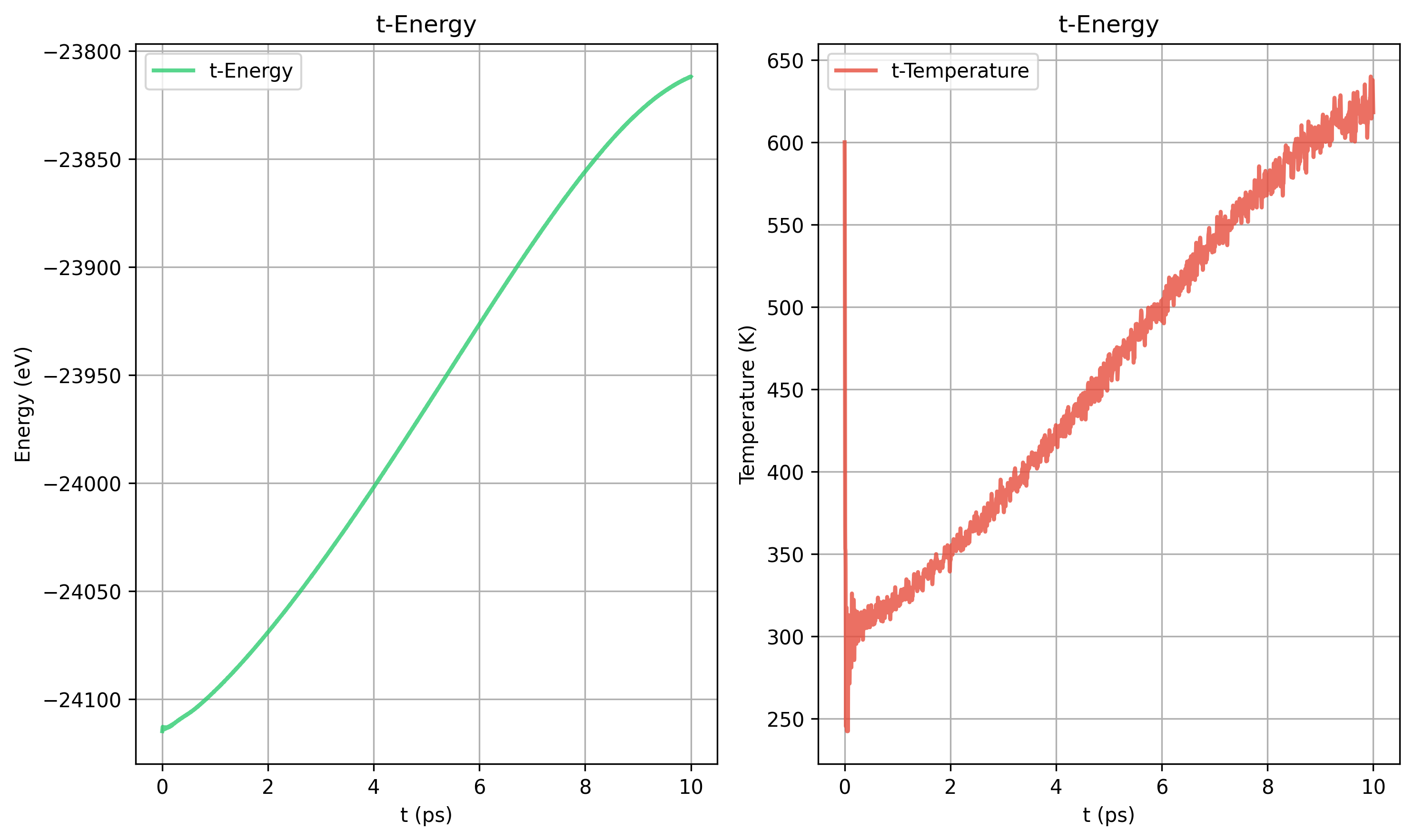
Nose-Hoover tdamp = 40 100 200 400 对比
40
100
200
400
from deepseek
9. 学习mattersim的phonon的方法
1. 包装ase的结构为phonon的格式
https://github.com/microsoft/mattersim/blob/main/src/mattersim/utils/phonon_utils.py
def to_phonopy_atoms(atoms: Atoms):
    """
    Transform ASE atoms object to Phonopy object
    Args:
        atoms (Atoms): ASE atoms object to provide lattice informations.
    """
    phonopy_atoms = PhonopyAtoms(
        symbols=atoms.get_chemical_symbols(),
        cell=atoms.get_cell(),
        masses=atoms.get_masses(),
        positions=atoms.get_positions(),
    )
    return phonopy_atoms


def to_ase_atoms(phonopy_atoms):
    """
    Transform Phonopy object to ASE atoms object
    Args:
        phonopy_atoms (Phonopy): Phonopy object to provide lattice informations.
    """
    atoms = Atoms(
        symbols=phonopy_atoms.symbols,
        cell=phonopy_atoms.cell,
        masses=phonopy_atoms.masses,
        positions=phonopy_atoms.positions,
        pbc=True,
    )
    return atoms
2. 修改mattersim以输出投影声子密度,并且指定固定的路径内的q点个数来匹配自己写的绘制声子谱的脚本(vasp模拟部分)(auto_band得到的q点个数在不同路径上不是固定的)
修改/lib/python3.12/site-packages/mattersim/applications/phonon.py
def compute_phonon_spectrum_dos(
        atoms: Atoms, phonon: Phonopy, k_point_mesh: Union[int, Iterable[int]]
    ):
        """
        Calculate phonon spectrum and DOS based on force constant matrix in
        phonon object

        Args:
            atoms (Atoms): ASE atoms object to provide lattice information
            phonon (Phonopy): Phonopy object which contains force constants matrix
            k_point_mesh (Union[int, Iterable[int]]): The qpoints number in First
                Brillouin Zone in three directions for DOS calculation.
        """
        print(f"Qpoints mesh for Brillouin Zone integration : {k_point_mesh}")
        phonon.run_mesh(k_point_mesh)
        print(
            "Dispersion relations using phonopy for "
            + str(atoms.symbols)
            + " ..."
            + "\n"
        )

        # plot phonon spectrum
        phonon.auto_band_structure(plot=True, write_yaml=True, with_eigenvectors=True).savefig(
            f"{str(atoms.symbols)}_phonon_band.png", dpi=300
        )
        phonon.auto_total_dos(plot=True, write_dat=True).savefig(
            f"{str(atoms.symbols)}_phonon_dos.png", dpi=300
        )

        # Save additional files
        phonon.save(settings={"force_constants": True})
主要修改了compute_force_constants 这个函数,替换为
# -*- coding: utf-8 -*-
import datetime
import os
from typing import Iterable, Union

import numpy as np
from ase import Atoms
from phonopy import Phonopy
from tqdm import tqdm
from seekpath import get_path
from phonopy.phonon.band_structure import get_band_qpoints_and_path_connections


from mattersim.utils.phonon_utils import (
    get_primitive_cell,
    to_ase_atoms,
    to_phonopy_atoms,
)
from mattersim.utils.supercell_utils import get_supercell_parameters


class PhononWorkflow(object):
    """
    This class is used to calculate the phonon dispersion relationship of
    material using phonopy
    """

    def __init__(
        self,
        atoms: Atoms,
        find_prim: bool = False,
        work_dir: str = None,
        amplitude: float = 0.01,
        supercell_matrix: np.ndarray = None,
        qpoints_mesh: np.ndarray = None,
        max_atoms: int = None,
        calc_spec: bool = True,
    ):
        """_summary

        Args:
            atoms (Atoms): ASE atoms object contains structure information and
                calculator.
            find_prim (bool, optional): If find the primitive cell and use it
                to calculate phonon. Default to False.
            work_dir (str, optional): workplace path to contain phonon result.
                Defaults to data + chemical_symbols + 'phonon'
            amplitude (float, optional): Magnitude of the finite difference to
                displace in force constant calculation, in Angstrom. Defaults
                to 0.01 Angstrom.
            supercell_matrix (nd.array, optional): Supercell matrix for constr
                -uct supercell, priority over than max_atoms. Defaults to None.
            qpoints_mesh (nd.array, optional): Qpoint mesh for IBZ integral,
                priority over than max_atoms. Defaults to None.
            max_atoms (int, optional): Maximum atoms number limitation for the
                supercell generation. If not set, will automatic generate super
                -cell based on symmetry. Defaults to None.
            calc_spec (bool, optional): If calculate the spectrum and check
                imaginary frequencies. Default to True.
        """
        assert (
            atoms.calc is not None
        ), "PhononWorkflow only accepts ase atoms with an attached calculator"
        if find_prim:
            self.atoms = get_primitive_cell(atoms)
            self.atoms.calc = atoms.calc
        else:
            self.atoms = atoms
        if work_dir is not None:
            self.work_dir = work_dir
        else:
            current_datetime = datetime.datetime.now()
            formatted_datetime = current_datetime.strftime("%Y-%m-%d-%H-%M")
            self.work_dir = (
                f"{formatted_datetime}-{atoms.get_chemical_formula()}-phonon"
            )
        self.amplitude = amplitude
        if supercell_matrix is not None:
            if supercell_matrix.shape == (3, 3):
                self.supercell_matrix = supercell_matrix
            elif supercell_matrix.shape == (3,):
                self.supercell_matrix = np.diag(supercell_matrix)
            else:
                assert (
                    False
                ), "Supercell matrix must be an array (3,1) or a matrix (3,3)."
        else:
            self.supercell_matrix = supercell_matrix

        if qpoints_mesh is not None:
            assert qpoints_mesh.shape == (3,), "Qpoints mesh must be an array (3,1)."
            self.qpoints_mesh = qpoints_mesh
        else:
            self.qpoints_mesh = qpoints_mesh

        self.max_atoms = max_atoms
        self.calc_spec = calc_spec

    def compute_force_constants(self, atoms: Atoms, nrep_second: np.ndarray):
        """
        Calculate force constants

        Args:
            atoms (Atoms): ASE atoms object to provide lattice informations.
            nrep_second (np.ndarray): Supercell size used for 2nd force
                constant calculations.
        """
        print(f"Supercell matrix for 2nd force constants : \n{nrep_second}")
        # Generate phonopy object
        phonon = Phonopy(
            to_phonopy_atoms(atoms),
            supercell_matrix=nrep_second,
            primitive_matrix="auto",
            log_level=2,
        )

        # Generate displacements
        phonon.generate_displacements(distance=self.amplitude)

        # Compute force constants
        second_scs = phonon.supercells_with_displacements
        second_force_sets = []
        print("\n")
        print("Inferring forces for displaced atoms and computing fcs ...")
        for disp_second in tqdm(second_scs):
            pa_second = to_ase_atoms(disp_second)
            pa_second.calc = self.atoms.calc
            second_force_sets.append(pa_second.get_forces())

        phonon.forces = np.array(second_force_sets)
        phonon.produce_force_constants()
        phonon.symmetrize_force_constants()

        return phonon

    @staticmethod
    def compute_phonon_spectrum_dos(
        atoms: Atoms, phonon: Phonopy, k_point_mesh: Union[int, Iterable[int]]
    ):
        """
        Calculate phonon spectrum and DOS based on force constant matrix in
        phonon object

        Args:
            atoms (Atoms): ASE atoms object to provide lattice information
            phonon (Phonopy): Phonopy object which contains force constants matrix
            k_point_mesh (Union[int, Iterable[int]]): The qpoints number in First
                Brillouin Zone in three directions for DOS calculation.
        """
        print(f"Qpoints mesh for Brillouin Zone integration : {k_point_mesh}")
        phonon.run_mesh(k_point_mesh)
        print(
            "Dispersion relations using phonopy for "
            + str(atoms.symbols)
            + " ..."
            + "\n"
        )
        #phonon.auto_band_structure(plot=True, write_yaml=True, with_eigenvectors=False).savefig(
           # f"{str(atoms.symbols)}_auto_band.png", dpi=300)

        lattice = atoms.cell
        scaled_positions = atoms.get_scaled_positions()
        atomic_numbers = atoms.get_atomic_numbers()
        path_data = get_path((lattice, scaled_positions, atomic_numbers))
        point_coords = path_data["point_coords"]
        band_segments = path_data["path"]

        from phonopy.phonon.band_structure import get_band_qpoints_and_path_connections
        raw_labels = []
        path = []
        connectionsall = []
        for start_label, end_label in band_segments:
            q_start = point_coords[start_label]
            q_end = point_coords[end_label]
            path.append([q_start,q_end])
            raw_labels.append(start_label)
            raw_labels.append(end_label)
            connectionsall.append('False')
        qpoints, connections = get_band_qpoints_and_path_connections(path, npoints=51)

        def convert_labels(raw_labels):
            latex_labels = []
            for label in raw_labels:
                if label.upper() == "GAMMA":
                    latex_labels.append("$\\Gamma$")
                else:
                    latex_labels.append(label)
            return latex_labels
        labels = convert_labels(raw_labels)
        phonon.run_band_structure(qpoints, path_connections=connections, labels=labels)
        bs = phonon.band_structure
        bs.write_yaml()
        plt = phonon.plot_band_structure()
        plt.savefig(f"{str(atoms.symbols)}_manual_band.png",dpi=300)


        phonon.auto_total_dos(plot=True, write_dat=True).savefig(
            f"{str(atoms.symbols)}_phonon_dos.png", dpi=300
        )
        phonon.auto_projected_dos(plot=True,write_dat=True).savefig(
            f"{str(atoms.symbols)}_phonon_projected_dos.png", dpi=300
        )
        phonon.save(settings={"force_constants": True})

    @staticmethod
    def check_imaginary_freq(phonon: Phonopy):
        """
        Check whether phonon has imaginary frequency.

        Args:
            phonon (Phonopy): Phonopy object which contains phonon spectrum frequency.
        """
        band_dict = phonon.get_band_structure_dict()
        frequencies = np.concatenate(
            [np.array(freq).flatten() for freq in band_dict["frequencies"]], axis=None
        )
        has_imaginary = False
        if np.all(np.array(frequencies) >= -0.299):
            pass
        else:
            print("Warning! Imaginary frequencies found!")
            has_imaginary = True

        return has_imaginary

    def run(self):
        """
        The entrypoint to start the workflow.
        """
        current_path = os.path.abspath(".")
        try:
            # check folder exists
            if not os.path.exists(self.work_dir):
                os.makedirs(self.work_dir)

            os.chdir(self.work_dir)

            try:
                # Generate supercell parameters based on optimized structures
                nrep_second, k_point_mesh = get_supercell_parameters(
                    self.atoms, self.supercell_matrix, self.qpoints_mesh, self.max_atoms
                )
            except Exception as e:
                print("Error whille generating supercell parameters:", e)
                raise

            try:
                # Calculate 2nd force constants
                phonon = self.compute_force_constants(self.atoms, nrep_second)
            except Exception as e:
                print("Error while computing force constants:", e)
                raise

            if self.calc_spec:
                try:
                    # Calculate phonon spectrum
                    self.compute_phonon_spectrum_dos(self.atoms, phonon, k_point_mesh)
                    # check whether has imaginary frequency
                    has_imaginary = self.check_imaginary_freq(phonon)
                except Exception as e:
                    print("Error while computing phonon spectrum and dos:", e)
                    raise
            else:
                has_imaginary = 'Not calculated, set calc_spec True'
                phonon.save(settings={"force_constants": True})

        except Exception as e:
            print("An error occurred during the Phonon workflow:", e)
            raise

        finally:
            os.chdir(current_path)

        return has_imaginary, phonon
转载请注明来源 有问题可通过github提交issue